Introduction to Quantum Programming Languages

Qiskit

Overview

Qiskit is an open source programming language developed by IBM and built on top of the Python programming language. It integrates with OpenQASM (with some hopefully temporary friction around OpenQASM versioning). In fact, Qiskit more accurately refers to a family of integrated frameworks for quantum computation. The most important of these are:

Qiskit Terra, a circuit description language with a Python-like syntax and the foundation of the Qiskit software stack. It also includes tools for the visualisation of circuits and quantum states, and for the optimisation of circuits for specific hardware devices.
Qiskit Aer, which provides facilities for classically simulating those circuits, along with realistic noise models for those simultations.

Along with classical simulations, Qiskit can also be used to interact with various quantum hardware providers in the cloud.

Tutorial

Qiskit is provided as a Pypi package for Python. As a result, its syntax follows the rules of Python. For starters, we import the package as usual:

import qiskit as qs

The core class for describing a quantum circuit in Qiskit is, unsurprisingly, the QuantumCircuit class. Its constructor takes up to two integer arguments, used to specify the number of quantum and classical registers (qubits and bits):

qc1 = qs.QuantumCircuit(4) # Construct a QuantumCircuit with 4 qubits
qc2 = qs.QuantumCircuit(4,3) # ... or with 4 qubits and 3 bits

We can then enact gates on the circuit by calling the corresponding methods of the class:

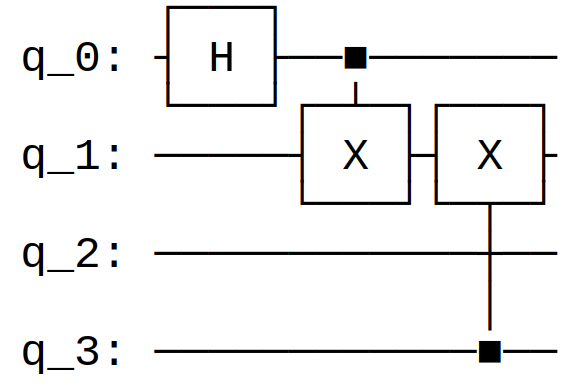
qc1.h(0)
qc1.cx(0,1)
qc1.cx(4,3)

We can then visualise this circuit with qc1.draw():

As you can see, the register of qubits is 0-indexed. Qiskit implements a large number of quantum gates in this way. Rather than listing them all here, we instead refer to the class documentation (or equivalently to calling help(qs.QuantumCircuit) within Python).

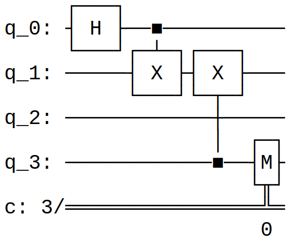
Measurements are a little different: they of course require access to a classical bit to store the outcome of the measurement.

qc2.h(0)
qc2.cx(0,1)
qc2.cx(4,3)

qc2.measure(2,0)

This results in the circuit:

We can then compose circuits with matching registers as follows:

qc3 = qs.QuantumCircuit(4)

qc3.cx(2,4)
qc3.cx(1,3)

qc1.compose(qc3).draw()

We can also build a QuantumCircuit whose quantum register is split into named subregisters. To understand this, we first need to introduce the QuantumRegister class, with an optional name:

qreg1 = qs.QuantumRegister(2,"register1")
qreg2 = qs.QuantumRegister(2,"register2")

ClassicalRegister has an analogous syntax for constructing classical registers. Then, we can build a QuantumCircuit from these registers:

qc3 = qs.QuantumCircuit(qreg1, qreg2)

qc3.h(0)
qc3.cx(qreg1[0],qreg1[1])
qc3.cx(qreg2[1],qreg2[0])

We can also initialise qubits with the following syntax:

qc3 = qc1.copy()
qc3.initialize([0,1], 2)

The first argument to initialize describes a qubit state as a pair of coefficients in the computational basis. The second argument describes the target qubit in the circuit for initialisation.

We can then compose circuits with matching registers:

qc4 = qs.QuantumCircuit(4)

qc4.cx(2,3)
qc4.cx(1,3)

qc1.compose(qc4)

Finally, we can output a QuantumCircuit to an OpenQASM 2.0 string using the qasm method.

Simulating and running quantum circuits

As described above, Qiskit also makes it possible to interact with various quantum hardward providers, as well as to run a simulation of a given quantum circuit on a classical backend. This allows one to extract (real or simulated) output states or outcome probabilites for measurements. The frontend for running circuits on actual quantum hardware is described in the documentation and depends on the provider in question.

We focus here on the classical simulation backends. These are provided via the qiskit.providers.aer submodule, specifically the AerSimulator class.

from qiskit.providers.aer import AerSimulator

In order to run the simulation, we need to set a initial state for each qubit. Here is an elementary example:

qc5 = qs.QuantumCircuit(1,0)
qc5.initialize([1,0],0)
qc5.h(0)

qc5.save_statevector()
simulator = AerSimulator()
qobj = qs.assemble(qc5, shots=1024)
result = simulator.run(qobj).result()
result.get_statevector()

with result:

Statevector([0.70710678+0.j, 0.70710678+0.j],
dims=(2,))

We can also get the resulting probabilities for different outcomes of a measurement in the computational basis:

result.get_counts()

Putting this all together, we can simulate the output state for one of our circuits for a given input state:

qc6 = qs.QuantumCircuit(4)
qc6.initialize([1,0],0)
qc6.initialize([1,0],1)
qc6.initialize([1,0],2)
qc6.initialize([1,0],3)
qc6 = qc6.compose(qc1)

qc6.save_statevector()
qobj = qs.assemble(qc6)
result = simulator.run(qobj).result() # Do the simulation and return the result
result.get_statevector()

This returns the result:

Statevector([0.70710678+0.j, 0.+0.j, 0.+0.j,
 0.70710678+0.j, 0.+0.j, 0.+0.j,
 0.+0.j, 0.+0.j, 0.+0.j,
 0.+0.j, 0.+0.j, 0.+0.j,
 0.+0.j, 0.+0.j, 0.+0.j,
 0.+0.j],
 dims=(2, 2, 2, 2))

If we add measurements to each qubit at the end of the circuit (using the measure_all method), we can then simulate outcome counts for the measurement. By default, these counts are made over 1024 simulated runs of the circuit.

qc6.measure_all()
qobj = qs.assemble(qc6)
result = simulator.run(qobj).result() # Do the simulation and return the result
result.get_counts()

Although the topic is beyond the scope of this tutorial, one of the main selling points of Qiskit Aer is that it provides realistic noise models for simulating quantum circuits run on NISQ devices.

Deutsch-Jozsa algorithm

For a complete explanation, see here.

# initialization
import numpy as np

# importing Qiskit
from qiskit import IBMQ, Aer
from qiskit.providers.ibmq import least_busy
from qiskit import QuantumCircuit, assemble, transpile

# import basic plot tools
from qiskit.visualization import plot_histogram

# set the length of the n-bit input string. 
n = 3

const_oracle = QuantumCircuit(n+1)

output = np.random.randint(2)
if output == 1:
const_oracle.x(n)

dj_circuit = QuantumCircuit(n+1, n)

# Apply H-gates
for qubit in range(n):
dj_circuit.h(qubit)

# Put qubit in state |->
dj_circuit.x(n)
dj_circuit.h(n)

dj_circuit = QuantumCircuit(n+1, n)

# Apply H-gates
for qubit in range(n):
dj_circuit.h(qubit)

# Put qubit in state |->
dj_circuit.x(n)
dj_circuit.h(n)

# Add oracle
dj_circuit += balanced_oracle

# Repeat H-gates
for qubit in range(n):
dj_circuit.h(qubit)
dj_circuit.barrier()

# Measure
for i in range(n):
dj_circuit.measure(i, i)

# Display circuit
dj_circuit.draw()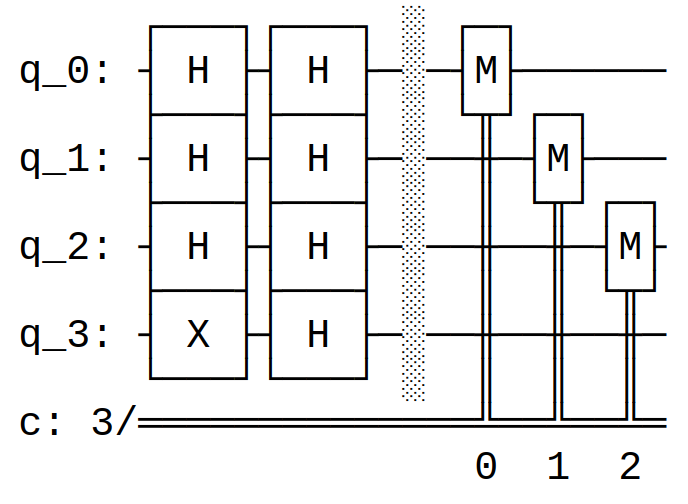

A range of Jupyter notebooks are also provided which give further examples of quantum computation in the language.

Back